Immune repertoire sequencing provides an extraordinary in-depth exploration of T and B cell receptors, which are crucial actors in human immunity. This has opened a vast number of research avenues in many fields and continues to do so. However, high-throughput sequencing data analysis can be challenging and requires data handling solutions that can deal with large data sizes, alignment of untemplated receptors, and error correction among others.
Accurate clone annotation is paramount to ensure the downstream analysis is sound and the results advance your research. That is why we developed our own gene annotation tool, designed to facilitate flexible, simple, scalable, and user-friendly analysis. When we came across a dataset that would allow us to verify the accuracy of our receptor annotation, we decided to give it a go and benchmark our gene annotation tool. The data comes from a publicly available benchmark dataset (Khan et al, Science Advances 2016) that includes a predefined mix of receptors, which are perfect for validation.
The dataset
The published AIRR (adaptive immune receptor repertoire) sequencing dataset consists of a set of 16 spike-ins that were specifically designed and synthesized to test immune repertoire sequencing and processing. In the original publication, these spike-ins were used as control sequences with distinct abundances so that any quantitative differences could be traced (so-called ‘amplification bias’). The spike-ins have been designed with unique CDR3 sequences so that they can be easily identified (see Table 1).
| CDR3 sequence | V gene | Frequency |
|---|---|---|
| CARIKKIVATYFDYW | IGHV1S81 | 23.38% |
| CWILLW | IGHV6-6 | 17.76% |
| CARMARKW | IGHV14-3 | 16.55% |
| CARLEDIW | IGHV2-9 | 16.17% |
| CARTARIKYW | IGHV3-2 | 8.59% |
| CARINAW | IGHV14-3 | 4.53% |
| CARSAIW | IGHV5-6-3 | 4.42% |
| CARSKYLARYW | IGHV2-9 | 2.39% |
| CARMARTINW | IGHV5-6-3 | 1.40% |
| CARTHERW | IGHV1-4 | 1.34% |
| CARLLINFDYW | IGHV1S81 | 1.28% |
| CTHERESAYW | IGHV6-6 | 0.69% |
| CARSIMANW | IGHV3-2 | 0.53% |
| CARVITRDYW | IGHV1S81 | 0.36% |
| CARKSTRASYW | IGHV1-4 | 0.34% |
| CRISTINAW | IGHV14-3 | 0.28% |
Table 1: Data from Khan et al, supplementary material, table S6. The quantification of the spike-ins has been performed with singleplex PCR. Please refer to the original publication for details.
The amplification steps before the sequencing were performed with a home-brew multiplex approach that introduces unique molecular identifiers (UMIs) in both the Forward and Reverse orientation (FID and RID, respectively). The authors use a custom method called Molecular Amplification Fingerprinting to analyze these spike-in samples and compensate for any quantitative differences that arise during amplification. Five technical replicates of the same spike-in mix were sequenced with MiSeq 2 x 300 bp. The primary data (fastq files) are available in SRA.
Processing with our gene annotation tool
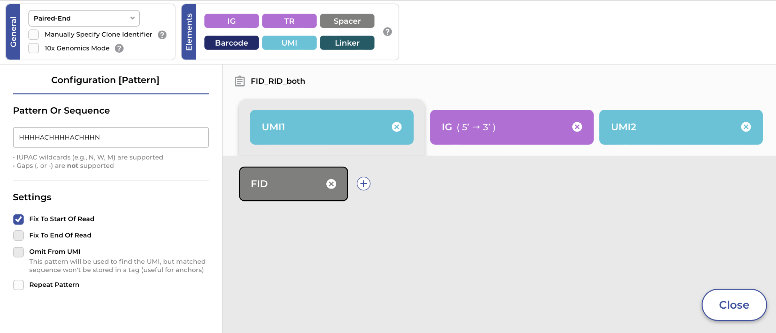
The five spike-in mix samples were obtained from SRA, uploaded onto the ENPICOM Platform, and processed with our gene annotation tool. Using the Sequence Template, we defined the amplicon structure that captured both FID (HHHHACHHHHACHHHN) and RID (NDDDDTGTDDDDDTGTDDDDDCAG) in the processing of the samples (Figure 1). Including these UMIs allowed for a better estimation of the original number of receptor sequences that were in the sample before amplification took place – providing more accurate clonal frequency results.
In addition to the UMI constructs, another consideration is the level of quality filtering to apply. This can be done in several ways, depending on specific issues that affect a dataset. Since this dataset appears to have a consistent quality and no other eyebrow-raising features, no QC filters or UMI cutoffs have been applied – any filtering step inevitably leads to fewer receptors being recovered, so in this case less really is more.
Using these FID and RID UMI constructs in the reads, with and without QC filters or UMI cutoffs, we recover slightly more immune receptors (~10%) from the raw sequencing data than the original publication did (see Table 2).
| Sample | Read pairs | Paper prod. reads | Our tool prod. reads | Reads > Q30 |
|---|---|---|---|---|
| SRR3175022 | 520308 | 64% | 78% | 77% |
| SRR3175024 | 651799 | 72% | 80% | 74% |
| SRR3175025 | 607690 | 68% | 77% | 76% |
| SRR3175026 | 695955 | 72% | 80% | 75% |
| SRR3175028 | 659047 | 66% | 76% | 75% |
Table 2: Processing stats from original publication (based on Table S1) and our gene annotation tool. Read pairs is the number of reads in the FASTQ files; reads > Q30 means the percentage of reads that have an average Phred score > 30.
Identification of spike-in sequences
The original publication highlights that many of the identified sequences were in fact mutated when compared to the original spike-ins. Furthermore, germline reference databases are updated frequently, so the V-gene annotations have likely diverged from the ones the researchers referred to. Therefore, we match the sequences from our processed output to the original spike-in sequences that we have obtained from the paper. This can be done in several ways, but for our purposes we choose two methods:
- Exact match by CDR3 amino acid sequence only – this is a lenient method and annotates ~90% of all sequences as spike-in sequences.
- Exact match by annotated spike-in receptor nucleotide sequence – this is a strict method that annotates ~60% of all sequences as spike-in sequences.
To match the nucleotide sequence of the spike-in, we compare the sequences from the processed receptors to those of Table S8 of the paper’s supplementary material. The spike-in receptor sequences are all 500nt long; the receptors recovered from the processed data are all shorter (336nt – 360nt), as expected. Thus, the requirement for a match is that the entire processed receptor sequence matches a section of the spike-in sequence from Table S8.
Regardless of using the lenient or strict methods, we are able to find all spike-ins in every sample – a promising initial step!
Comparing sample counts to spike-in frequencies
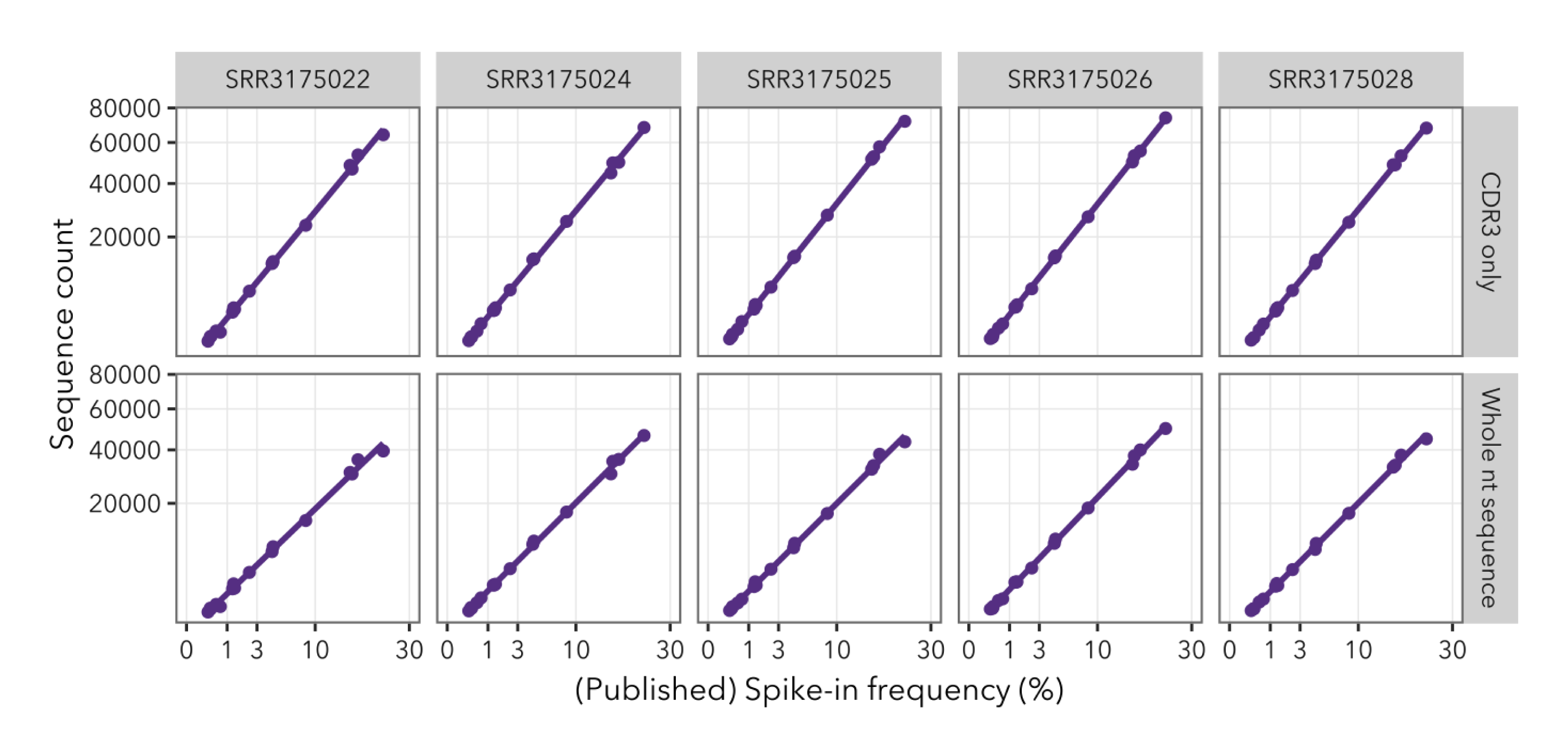
With the spike-ins mapped, we compared them to the original spike-in frequencies, depicted in Figure 2. The spike-in counts as quantified by our gene annotation tool are mapped against the original spike-in frequencies from the paper, separately for all 5 replicates. The processed results align very well with the original frequencies, both for the lenient (CDR3 only) and the strict (whole nt sequence) spike-in annotation method. Note that the differences in counts are due to the different number of read pairs that are in the samples (see also Table 2).
Comparing our gene annotation tool to the original paper’s MAF method
So how does our gene annotation tool compare to the original MAF method? This method is introduced in the paper specifically for recovering the original spike-in frequencies. Briefly, the MAF method applies a custom mathematical model to the forward and the reverse UMI counts (FID and RID, respectively) to compensate for amplification biases that may have been introduced during library preparation and sequencing. The MAF method thus provides a more accurate estimate of sequence counts than do uncompensated counts, as the original results show in Khan et al, Figure 4. Our gene annotation tool uses UMI processing to achieve the same goal, and hence we can compare these two analysis tools for their ability to compensate for amplification biases in these samples.
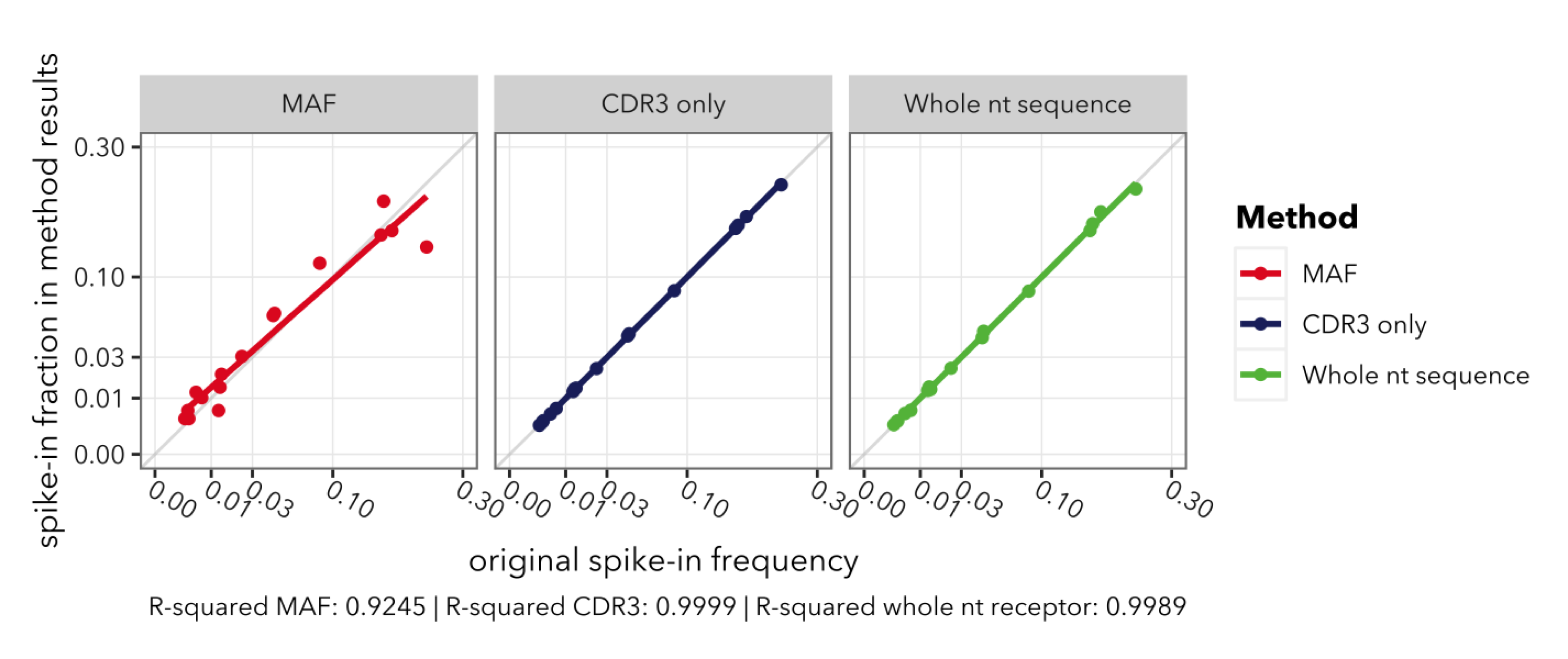
Conveniently, the average MAF mean and standard deviation (sd) values are given in the paper (Table S6). To compare the methods, all values are re-normalized into count fractions to compensate for differences in read pairs per sample, percentage productive reads (our gene annotation tool is a bit more sensitive), and method count ranges. The normalized values should therefore match the original spike-in fractions and line up on the y = x diagonal – that is, if the methods fully recover the quantitative differences between the spike-in sequences. The results are depicted in Figure 3. The plots show that both of our tool’s methods line up with the diagonal almost perfectly – 4 digits are required to see the difference between them. The MAF approach does not achieve the same accuracy but fits still well with an R² of 0.9245. Additionally, we see that the regression lines of our tool’s fits are closer to the diagonal; the slopes of our tool’s fractions are spot-on (both 1), while MAF’s is 0.89, indicating that it overestimates the counts of lower-frequency spike-ins – or an underestimation of the higher-frequency spike-ins.
Coefficient of variation
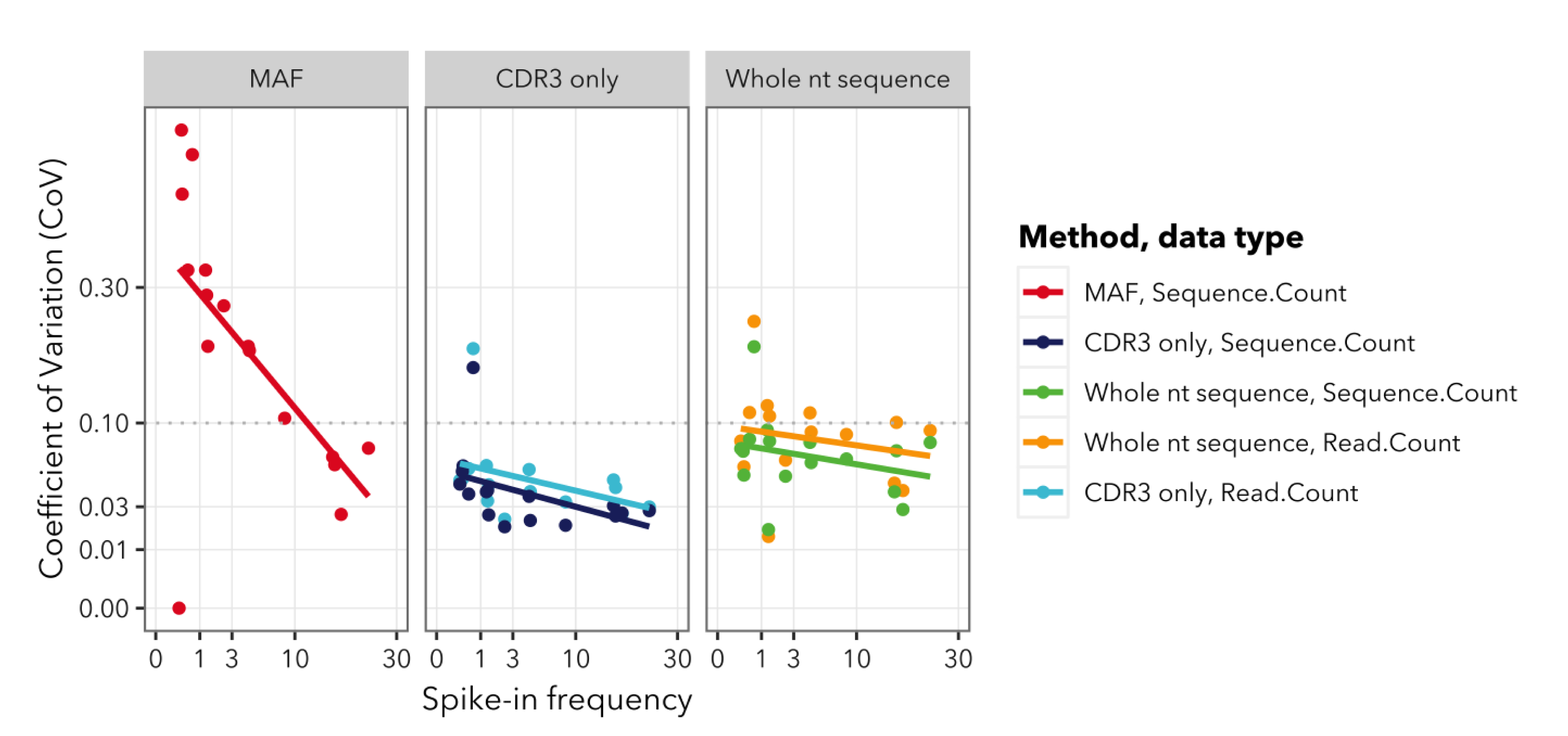
Finally, we decided to compare the precision of the normalized counts using the coefficient of variation (CoV), which is the standard deviation divided by the mean. This is a measure of how much signal is obtained relative to the variability in the outcome (I guess some call it ‘noise’). For CoV: lower is better, we want as little variation and as much signal as possible. The values are plotted in Figure 4.
For all methods, we see a few expected trends. For instance, the CoV is lower for high-abundance sequences; conversely, low-abundance measurements have more variability which is a common feature of NGS data. Furthermore, we see that the CoV is larger for raw read counts (plotted as Read Count) than for counts that have been corrected using FID and RID (UMI) processing (plotted as Sequence Count). This is consistent with the UMIs effect on sequence quantification accuracy.
We see that the CoV is lowest for the CDR3 matching approach. This is probably due to the higher counts obtained (more spike-in matches in the sample) that are present in this approach, which increase the mean but have no significant effect on the variation. Furthermore, we see that the CoV values for data processed by our gene annotation tool are generally lower than the MAF values. To quantify this, we can use an (arbitrary) cutoff of 0.1 (dotted grey line in Figure 4) and quantify how many points are under this line. We see that with the MAF method from the paper, five spike-ins have a CoV of lower than 0.1, and eleven do not. With our gene annotation tool, even for the ‘Full nt sequence’-approach and with Read Count, we see that ten spike-ins have a CoV lower than 0.1 and six do not. For all other quantification methods of our gene annotation tool in all samples, the CoV is under the 0.1 threshold for all spike-ins except one. This indicates that using UMI with our gene annotation tool gives a lower variance compared to other methods, even if these are based on more complex UMI configurations.
Outcomes
So, what have we learned after this quick spike-in analysis?
- It was easy to reprocess these benchmark samples due to our gene annotation tool’s flexible configuration that captured both the spike-ins and complex UMI’s they contained.
- Our gene annotation tool identified more spike-in sequences with higher accuracy than the original MAF method. This is independent of how the spike-ins are annotated: both with a lenient and with a strict matching method, the results are better than the original.
- Analysis of the coefficient of variation shows that the use of UMI for reducing amplification bias and error correction improves the precision of quantification.
All in all, this re-analysis demonstrates the rapid advancements being made in repertoire sequencing. Many of the challenges faced in the past have been largely overcome, resulting in a technology providing more accurate and reliable results compared to those achievable just a few years ago.
Interested to learn how it can be applied in your research? Talk to our experts today!